In the complex landscape of digital systems, understanding the flow of signals is paramount. Timing diagrams serve as the visual language that engineers use to describe the behavior of signals over time. Whether you are designing hardware logic or analyzing software threads, these diagrams provide the clarity needed to ensure that operations occur in the correct sequence. This guide explores the mechanics of timing diagrams, focusing heavily on how they illustrate concurrency and synchronization within a system.

What Is a Timing Diagram? 📊

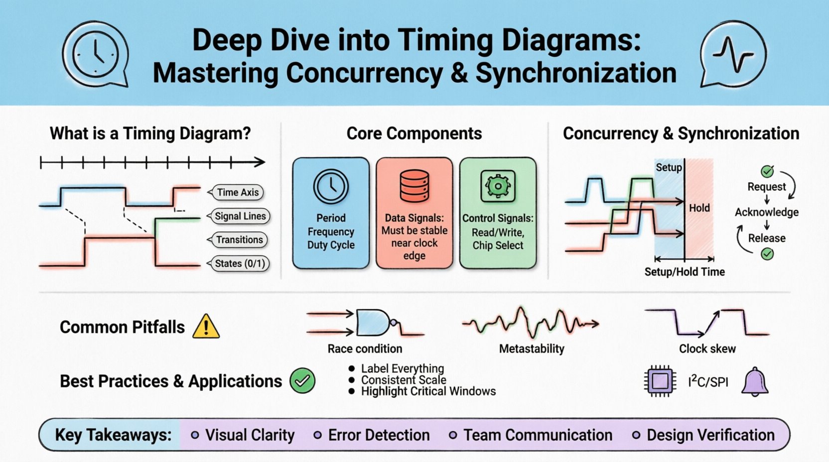
A timing diagram is a graphical representation that shows the relationship between two or more signals as they change over time. It is a fundamental tool in system design, used to verify that data transfers, control signals, and clock cycles align properly. Without this visual aid, debugging asynchronous behavior becomes nearly impossible.

• Time Axis: Typically runs horizontally from left to right.
• Signal Lines: Represent individual wires, buses, or logical states.
• Transitions: Vertical lines indicate changes from high to low or vice versa.
• States: Defined by the logic level (0, 1, High, Low) at any given moment.

These diagrams are not merely pictures; they are specifications. They define the allowable window of time for a signal to be valid before the next clock edge arrives. This precision is critical for preventing data corruption.

Core Components of Timing Diagrams ⚙️

To read these diagrams effectively, one must understand the specific elements that make them up. Each component carries specific meaning regarding the timing constraints of the system.

1. Clock Signals 🕰️

The clock signal acts as the heartbeat of the system. It dictates when data should be sampled or latched. In synchronous systems, all actions are triggered by the rising or falling edge of this clock.

• Period: The duration of one complete cycle.
• Frequency: The number of cycles per second (Hz).
• Duty Cycle: The percentage of time the signal remains high versus low.

2. Data Signals 💾

Data lines carry the actual information being processed. Their state must remain stable for a specific duration relative to the clock edge. This stability is what timing diagrams analyze.

3. Control Signals 🎛️

These signals manage the flow of data. Examples include read/write enable, chip select, or interrupt requests. They often dictate when data lines are allowed to change state.

Concurrency in System Design 🔄

Concurrency refers to the ability of a system to execute multiple processes or threads simultaneously. In hardware, this might mean multiple buses accessing memory. In software, it implies multiple threads running on a CPU core.

Why Concurrency Matters

Modern systems rely on concurrency to maximize throughput and efficiency. However, introducing multiple active paths increases the risk of conflicts. Timing diagrams help visualize these potential conflicts.

• Parallel Execution: Multiple operations happening at the same time.
• Resource Sharing: Multiple threads accessing the same memory location.
• Latency Variations: Different paths taking different amounts of time.

Visualizing Concurrent Signals

When drawing a timing diagram for a concurrent system, you stack the signal lines vertically. This allows you to see overlaps. If two signals claim control of a bus at the same time, the diagram will show overlapping active states, indicating a potential collision.

Synchronization Mechanisms ⏱️

Synchronization ensures that concurrent processes coordinate their actions so that they do not interfere with one another. Timing diagrams are the primary tool for verifying that synchronization protocols are met.

1. Setup and Hold Times ⏲️

These are the most critical timing constraints in digital logic. They define the window in which input data must be stable relative to the clock edge.

Parameter	Definition	Consequence of Violation
Setup Time	Time before the clock edge that data must be stable	Metastability or incorrect data capture
Hold Time	Time after the clock edge that data must remain stable	Data corruption or race conditions

Violating these constraints can lead to metastability, where a flip-flop enters an undefined state. Timing diagrams must explicitly mark these windows to ensure design compliance.

2. Handshake Protocols 🤝

Asynchronous systems often use handshakes to synchronize data transfer without a global clock. The sender asserts a signal, waits for an acknowledgment from the receiver, and then proceeds.

• Request: Signal indicating data is ready.
• Acknowledge: Signal confirming receipt.
• Release: Signal returning to idle state.

A timing diagram for a handshake will show a sequence of pulses. If the acknowledgment does not arrive before the request timeout, the sender must retry. The diagram helps identify if the timeout is set correctly.

Reading and Interpreting Signals 📈

Interpreting a timing diagram requires attention to detail. You must look for edges, levels, and delays.

Edge Detection

Edges represent changes. A rising edge might trigger a latch, while a falling edge might clear a register. In diagrams, these are sharp vertical transitions.

• Rising Edge: Low to High transition.
• Falling Edge: High to Low transition.
• Glitch: A short, unintended pulse that might cause errors.

Signal Delays ⏳

No signal travels instantly. Propagation delay occurs between the source and the destination. On a timing diagram, this is visible as a horizontal gap between the source transition and the destination transition.

Understanding these delays is crucial for calculating the maximum frequency of the system. If the delay is too long, the clock period must be increased (frequency decreased) to allow signals to settle.

Common Challenges and Pitfalls ⚠️

Even experienced engineers encounter issues when designing or analyzing timing. Recognizing common pitfalls helps prevent costly errors in the final product.

1. Race Conditions

A race condition occurs when the system behavior depends on the sequence or timing of events that are not controlled. If two signals arrive at a logic gate at slightly different times, the output might be unpredictable.

• Positive Race: One signal arrives faster than expected.
• Negative Race: One signal arrives slower than expected.

2. Metastability

This happens when a flip-flop receives a data input that violates setup or hold times. The output enters an oscillating state before settling to 0 or 1. This can propagate errors through the entire system.

3. Skew

Clock skew occurs when the clock signal arrives at different components at different times. This reduces the effective setup and hold margins. Timing diagrams must account for the worst-case skew between any two elements.

Best Practices for Accuracy ✅

To ensure your timing diagrams are reliable and useful, follow these guidelines.

• Label Everything: Include time markers, signal names, and voltage levels.
• Use Consistent Scale: Ensure the time axis is linear and clearly marked.
• Highlight Critical Windows: Use shading or colors to mark setup and hold times.
• Document Assumptions: Note any clock frequencies or propagation delays assumed in the diagram.
• Verify with Simulation: Always cross-reference diagrams with simulation waveforms.

Real-World Applications 🌍

Timing diagrams are used across various domains. From embedded microcontrollers to high-speed network protocols, the principles remain the same.

1. Memory Interfaces

In DDR memory, timing is extremely tight. Diagrams show the relationship between the clock, data, and command lines. Setup and hold times are critical here to prevent data corruption during high-speed transfers.

2. Communication Protocols

Protocols like I2C, SPI, and UART rely on specific timing. For example, I2C requires the SDA line to be stable when the SCL line is high. A timing diagram makes these rules explicit.

3. Interrupt Handling

When an interrupt occurs, the system must pause current tasks and execute an interrupt service routine. Timing diagrams show the latency between the interrupt request and the start of the routine.

Advanced Techniques for Analysis 🔬

For complex systems, basic diagrams may not suffice. Advanced techniques allow for deeper analysis of signal integrity and timing closure.

1. Static Timing Analysis (STA)

STA calculates the worst-case delays without running simulations. It uses the timing diagram as a reference to verify that all paths meet the clock period constraints. It checks for hold violations and setup violations across all process corners.

2. Dynamic Timing Analysis

This involves running simulations to observe actual signal behavior. It captures glitches and glitches that static analysis might miss. It provides a realistic view of how signals behave under load.

3. Clock Domain Crossing (CDC)

When signals move between different clock domains, synchronization is required. Timing diagrams help visualize the metastability window and the need for synchronizer chains.

Summary of Key Takeaways 📝

Timing diagrams are essential for visualizing the temporal relationships between signals in a system. They are the bridge between abstract logic and physical implementation.

• Visual Clarity: They make abstract timing constraints concrete.
• Error Detection: They help identify race conditions and metastability risks.
• Communication: They serve as a common language between hardware and software engineers.
• Design Verification: They validate that the system meets performance requirements.

By mastering the art of reading and creating these diagrams, engineers can build more reliable, efficient, and robust systems. The investment in understanding these visual tools pays off in reduced debugging time and higher system stability.

Final Thoughts on System Reliability 🛡️

Reliability is the cornerstone of any engineering project. Timing diagrams provide the evidence needed to prove that a design will function correctly under all conditions. They force the designer to think about time, not just logic.

As systems become faster and more complex, the importance of precise timing analysis only grows. Whether dealing with nanosecond precision in hardware or millisecond delays in network protocols, the principles of concurrency and synchronization remain constant.

Remember to always verify your diagrams against real-world measurements. Simulations are great, but they are models. Real signals have noise, impedance, and capacitance that affect timing. Use diagrams as a planning tool, but validate with measurement.

With a solid grasp of timing diagrams, you are equipped to tackle the challenges of modern system design. Focus on the constraints, respect the edges, and always plan for the worst-case scenario.