In the intricate world of embedded systems and digital design, logic stability is not merely a preference; it is a requirement. Firmware serves as the intelligence behind the silicon, dictating how hardware responds to external stimuli. However, the complexity of modern microcontrollers and application-specific integrated circuits (ASICs) often leads to subtle bugs that are difficult to trace. The most robust approach to mitigating these issues lies in the disciplined application of two fundamental tools: timing diagrams and finite state machines (FSMs). Together, they form a rigorous framework for designing firmware that is predictable, verifiable, and maintainable.

Understanding the relationship between signal timing and logical state is crucial for any engineer working on sequential logic. When these two concepts are aligned, the resulting firmware behaves consistently across temperature variations, voltage fluctuations, and clock speed changes. This guide explores how to leverage these tools to create reliable firmware logic without relying on guesswork or trial-and-error debugging.

📈 The Foundation: Understanding Timing Diagrams

A timing diagram is a graphical representation of how signals change over time. It is the primary language used to communicate temporal relationships between hardware components and firmware routines. In the context of firmware logic, these diagrams act as a contract between the hardware environment and the code executing upon it.

Key Elements of a Timing Diagram

• Time Axis: Represents the progression of clock cycles or absolute time. It establishes the rhythm at which the system operates.
• Signal Lines: Horizontal lines representing specific inputs, outputs, or internal flags. Each line corresponds to a bit or a group of bits.
• Edges: Vertical transitions indicating rising edges (low to high) or falling edges (high to low). These often trigger state changes.
• High/Low States: The logical levels maintained between transitions, defining the data value at any given moment.
• Delays: Gaps between events, such as setup time, hold time, or propagation delay, which dictate the minimum time required for stability.

When designing firmware, a timing diagram answers the question: “When is data valid?” and “When should the system react?” Without this visual context, logic design becomes a guessing game. For example, if a sensor signal is sampled too early, before it has settled, the firmware will read garbage data. If it is sampled too late, it might miss a pulse entirely.

Why Timing Diagrams Matter in Firmware

• Clarification of Hardware Constraints: They explicitly show setup and hold times required by peripheral devices.
• Debugging Reference: When a system fails, a timing diagram provides a baseline for expected behavior versus actual behavior.
• Communication: They serve as a universal document for hardware and software teams to agree on interface protocols.
• Optimization: They help identify bottlenecks where software waits unnecessarily for hardware signals.

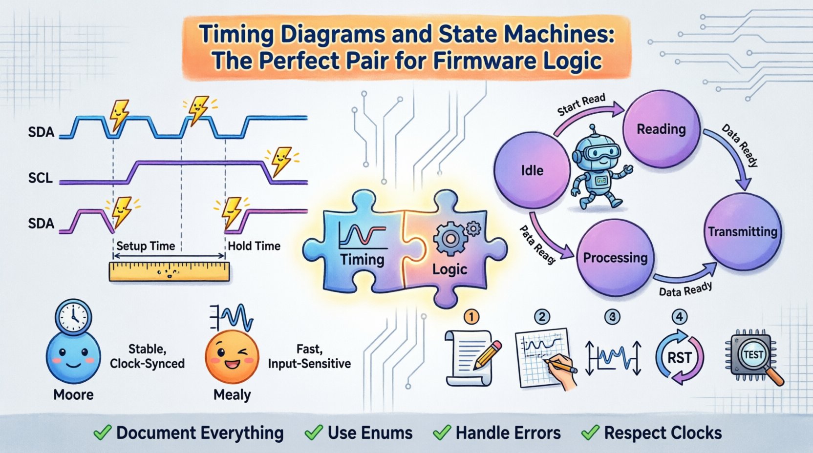
Consider a scenario involving an I2C communication interface. The firmware must wait for the clock line to stabilize before reading data. A timing diagram visually maps out the SDA and SCL lines, showing exactly where the start condition, address byte, and data byte occur. This visualization prevents race conditions where the software might attempt to read the data bus while the master is still driving the clock.

🔄 The Logic Engine: Finite State Machines (FSMs)

While timing diagrams define the environment, the Finite State Machine defines the behavior. An FSM is a model of computation used to design both computer programs and sequential logic circuits. It consists of a finite number of states, transitions between those states, and actions.

Components of a State Machine

• State: A snapshot of the system at a specific moment. It represents the current mode of operation (e.g., Idle, Reading, Processing, Transmitting).
• Transition: The movement from one state to another based on specific conditions or inputs.
• Input: External signals or internal flags that trigger a state change.
• Output: Actions or signals generated while in a specific state (Moore) or during a transition (Mealy).

Moore vs. Mealy Machines

Selecting the right type of state machine is a critical design decision. The choice impacts timing sensitivity and output stability.

Feature	Moore Machine	Mealy Machine
Output Dependency	Depends only on the current state	Depends on current state and input
Timing Stability	More stable; outputs change only on clock edge	Faster response; outputs can change immediately with input
Complexity	May require more states to handle specific input combinations	Often requires fewer states for the same functionality
Glitch Sensitivity	Less sensitive to input glitches	More sensitive to input glitches

For firmware logic where signal integrity is paramount, Moore machines are often preferred. Because outputs are tied strictly to the state and typically synchronized to the clock edge, they reduce the risk of asynchronous glitches propagating through the system. Mealy machines offer speed but require careful timing analysis to ensure inputs do not introduce metastability.

🤝 Synchronizing Timing and Logic

The true power of this pairing lies in the synchronization of the timing diagram with the state machine transition logic. Every transition in the state machine must correspond to a valid point in the timing diagram. If the hardware signal changes at a time that conflicts with the clock cycle, the firmware may enter an undefined state.

Establishing the Clock Domain

All state transitions should ideally occur on a specific clock edge (usually the rising edge). The timing diagram must show that all input signals are stable during the setup time before the clock edge and remain stable during the hold time after the clock edge. Firmware logic that ignores these windows risks sampling incorrect data.

To ensure this alignment:

• Map Inputs to Clock Cycles: Define exactly which clock cycle an input will be sampled. Do not sample an input arbitrarily within a cycle.
• Debounce Inputs: Mechanical switches or noisy sensors require time to settle. The timing diagram should include debounce windows, and the state machine should have a dedicated “Waiting” state to handle this period.
• Avoid Combining Asynchronous Events: If an interrupt occurs, it must be synchronized to the system clock before entering the state machine logic.

Handling Asynchronous Inputs

Not all signals are synchronous to the system clock. External interrupts, sensor triggers, or user inputs may arrive at random times. When these signals interact with a clocked state machine, the timing diagram becomes the safety net.

The standard technique involves a multi-stage synchronizer. The timing diagram should illustrate the signal passing through two or more flip-flops, allowing it to settle before being read by the state machine. This prevents metastability, a condition where the signal is neither a logical 0 nor 1, causing the system to hang or crash.

🛠️ Implementation Workflow

Developing firmware using this paired approach requires a structured workflow. Skipping steps often leads to fragile code that is difficult to maintain. The following steps outline a professional methodology for integrating timing diagrams and state machines.

1. Define the Protocol and Constraints

Before writing a single line of code, document the timing requirements. Create a timing diagram that represents the ideal behavior. Include minimum pulse widths, maximum response times, and idle states. This document serves as the source of truth for the firmware logic.

2. Design the State Machine Topology

Sketch the state diagram. Identify all possible states and the conditions required to transition between them. Ensure that every state has a defined exit condition. Avoid “orphan” states where the system can get stuck indefinitely.

3. Map Logic to Timing

Align the state transitions with the clock edges defined in the timing diagram. For example, if a state machine needs to wait for a 10-millisecond delay, calculate how many clock cycles this represents at the current system frequency. Implement this as a counter within the state, rather than a software delay loop that blocks the processor.

4. Implement Reset Logic

A robust firmware must return to a known state upon reset. The timing diagram should indicate the reset signal duration. The state machine initialization code must ensure that the system starts in the defined “Idle” or “Ready” state, regardless of the power-up sequence.

5. Verification and Simulation

Simulate the logic against the timing diagram. Check for violations where the software assumes a signal is valid when it is not. Look for race conditions where the state changes faster than the hardware can respond. Use generic simulation environments to model the hardware behavior and verify the firmware logic against the timing constraints.

🔍 Debugging and Verification

Even with careful planning, issues arise. When firmware logic fails, the combination of timing diagrams and state machines provides a powerful debugging strategy. Instead of random logging, use these tools to isolate the failure point.

Common Timing Violations

• Setup Time Violation: The data input changed too close to the clock edge. The firmware reads unstable data. Solution: Shift the sampling point in the state machine to a later cycle.
• Hold Time Violation: The data input changed too soon after the clock edge. The flip-flop loses the previous state. Solution: Add buffering or delay in the hardware path.
• Metastability: The signal is unresolved. The system may behave erratically. Solution: Implement a proper two-stage synchronizer.

State Machine Errors

• Unreachable States: States that cannot be entered or exited. These usually indicate logic errors in the transition conditions.
• Spurious Transitions: The system enters a state it shouldn’t due to noise. Solution: Add input validation or debouncing states.
• Infinite Loops: The system stays in one state forever. Solution: Ensure all states have a timeout or exit condition.

Using the Diagram for Root Cause Analysis

When a bug occurs, overlay the actual signal traces onto the ideal timing diagram. Look for deviations. Did the input signal arrive late? Did the clock jitter? Did the state machine transition prematurely? This visual comparison narrows the search space significantly compared to reading raw code logs.

📊 Best Practices for Robust Logic

To maintain high quality and reliability over the lifecycle of a project, adhere to these best practices. These guidelines help prevent technical debt and ensure the firmware remains adaptable.

• Document Everything: Keep the timing diagrams and state diagrams updated alongside the code. Outdated documentation is worse than no documentation.
• Keep States Simple: Avoid complex state machines with too many branches. If a machine has more than 10 states, consider breaking it into sub-machines.
• Use Explicit Enums: Define state names as constants or enumerations. Avoid using magic numbers like “if (state == 3)”. Use “if (state == STATE_IDLE)”.
• Handle Errors Gracefully: Include an “Error” state. If the system detects an invalid condition, transition to this state and halt or reset, rather than continuing with undefined logic.
• Respect Clock Domains: If the system uses multiple clock frequencies, implement proper clock domain crossing techniques. Never move data directly between asynchronous clocks.
• Minimize Blocking Delays: Do not use “while” loops that wait for time to pass. Use the state machine to manage time using counters, allowing the processor to handle other tasks.

🔗 Real-World Application Example

Consider a simple battery management system. The firmware monitors voltage, controls charging current, and communicates status to a host computer.

State 1: Idle. The system waits for a charge request signal. The timing diagram shows this signal must be high for at least 5 milliseconds.

State 2: Charging. Upon valid request, the system enters charging. A timer state ensures the current flows for a specific duration. If the voltage exceeds the limit, the system transitions to State 3: Over-Voltage Protection.

State 3: Protection. The charging circuit is disabled. The system waits for the voltage to drop below a safe threshold before returning to Idle. A timing diagram ensures the voltage sensor is sampled only after the protection hardware has physically disconnected the load.

Without the state machine, the code might check voltage in a continuous loop. If the voltage spikes briefly, the loop might react too fast, causing oscillation. With the state machine, the transition to Protection requires a stable condition over time, preventing false triggers.

🚀 Moving Forward

The integration of timing diagrams and state machines is not just a design choice; it is a discipline that separates functional code from production-ready firmware. By visually defining the temporal constraints and structurally defining the logical flow, engineers create systems that are resilient to noise, hardware variations, and operational stress.

This approach requires upfront effort. It demands time to draw diagrams and plan states before coding begins. However, the cost of debugging a race condition in the field far exceeds the cost of designing it correctly initially. As systems become more complex, the need for this structured methodology grows. There is no shortcut to reliability. The path forward involves continuous documentation, rigorous verification, and a respect for the timing constraints of the physical world.

Adopting these practices ensures that the firmware logic remains transparent and testable. It allows teams to collaborate effectively, knowing that the timing diagrams define the reality in which the state machines operate. In an industry where hardware is expensive and time-to-market is critical, this pairing offers the best chance for success.

✅ Key Takeaways

• Timing diagrams provide the visual contract for signal behavior over time.
• State machines provide the structured logic for system behavior.
• Synchronization is the critical link between the two tools.
• Moore machines offer better timing stability than Mealy machines for most embedded tasks.
• Debugging is most effective when actual traces are compared against the ideal timing diagram.
• Documentation must evolve with the code to remain useful.

By adhering to these principles, firmware engineers can build logic that stands the test of time, ensuring stability in an increasingly complex digital landscape.