When engineers discuss embedded systems, the term asynchronous often triggers a specific mental model. Many assume that if a design is asynchronous, time is irrelevant. They picture a world where signals change at will, unbound by clocks, and completely free from timing constraints. This is a dangerous misconception. In reality, asynchronous design is deeply rooted in time. It is simply a different way of managing it. Understanding this distinction is critical for anyone working with timing diagrams, signal integrity, or low-power architecture.

The reality is stark: time is a physical constant in electronics. Electrons take time to travel through a wire. Logic gates take time to switch states. If you assume timing does not exist, you risk building a system that fails unpredictably. This article dissects the relationship between asynchrony and timing, focusing on how timing diagrams remain the single most important tool for verification, regardless of the clock strategy.

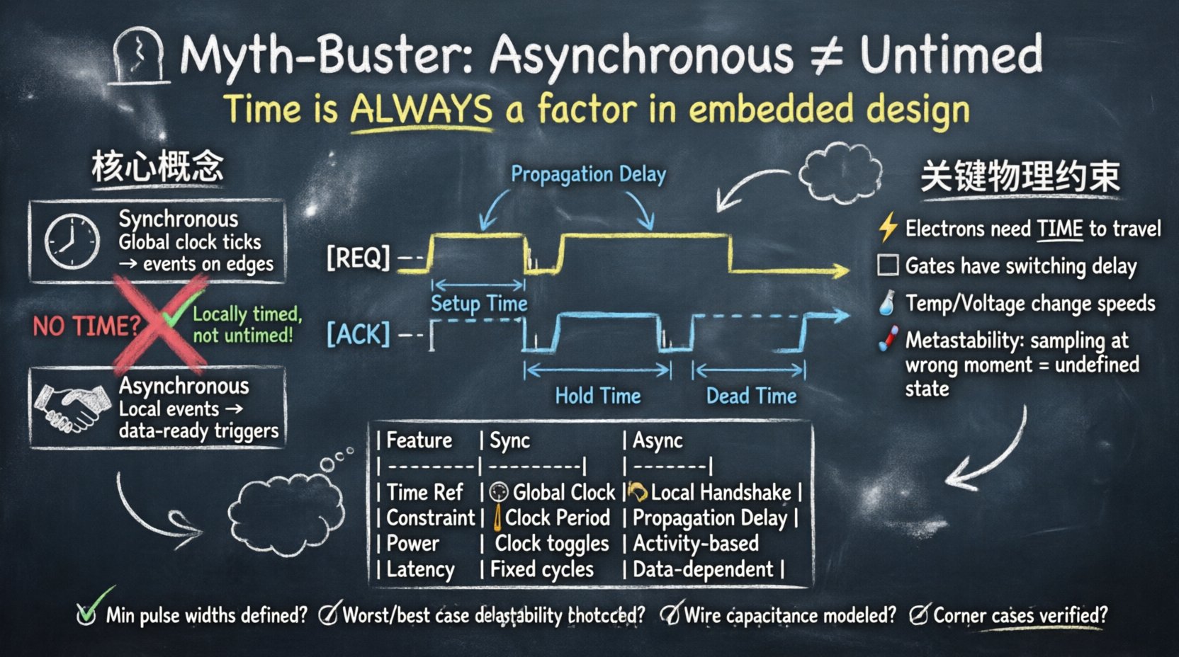
The Core Misconception: Time vs. Clocks 🕰️

The confusion stems from the vocabulary used in digital logic. In synchronous design, a global clock signal dictates when data is sampled. Everyone moves in lockstep. This makes it easy to visualize time. You look at the clock edge, and you know exactly when the next event can happen.

In asynchronous design, there is no global clock. Instead, local signals trigger events. This is often called event-driven or self-timed. Because the concept of a “tick” disappears, some designers incorrectly assume the concept of duration disappears too. They are wrong.

Here is the breakdown of the difference:

• Synchronous Design: Time is quantized by the clock period. Operations happen on edges.
• Asynchronous Design: Time is continuous. Operations happen when data arrives and validation completes.

Even without a clock, signals must transition within specific windows. If a signal arrives too early, the receiver might not be ready. If it arrives too late, the receiver might have already moved on. These windows are defined by timing diagrams. Therefore, asynchronous logic is not untimed; it is locally timed.

Physical Reality: Propagation and Latency ⚡

Regardless of the design methodology, the laws of physics apply. A logic gate is not an abstract switch. It is a physical circuit made of transistors. When a voltage changes, it must overcome capacitance and resistance. This creates propagation delay.

Consider an asynchronous handshake protocol, such as the Request-Acknowledge (REQ-ACK) scheme. This is common in FIFOs and communication interfaces.

• Request Phase: The sender asserts a line to indicate data is ready.
• Processing Phase: The receiver reads the data and processes it.
• Acknowledge Phase: The receiver signals that data has been accepted.
• Reset Phase: The sender deasserts the line to prepare for the next transaction.

Every single one of these phases requires a specific amount of time. If the sender deasserts the request before the receiver has fully captured the acknowledge signal, data corruption occurs. This is not a theoretical risk; it is a physical constraint. Timing diagrams are used to map these intervals. They show the minimum pulse widths required for the circuit to recognize a state change.

Without a clock to enforce margins, the designer must rely on delay models. These models estimate how long a signal takes to travel from point A to point B. If the delay is underestimated, the system races. If overestimated, performance suffers. Timing diagrams visualize these delays as horizontal distances between signal edges.

The Anatomy of a Timing Diagram in Async Systems 📊

In synchronous design, a timing diagram looks like a grid. In asynchronous design, the grid disappears, but the measurement lines remain. A timing diagram for an asynchronous interface focuses on relative relationships rather than absolute clock cycles.

Key elements to analyze in an asynchronous timing diagram include:

• Signal Edges: Rising and falling transitions are the triggers. The exact moment matters.
• Hold Time: How long must a signal stay stable after a transition? In async, this is often critical for latch-based storage.
• Setup Time: How long must data be stable before a transition occurs? This ensures the receiver has time to capture the value.
• Dead Time: The period where no activity occurs between transactions. This impacts power consumption.
• Overlap: The period where request and acknowledge signals are both active. Too much overlap causes contention.

When reading these diagrams, you are looking for causality. In a clocked system, causality is enforced by the clock edge. In an async system, causality is enforced by the logic gates themselves. The timing diagram must prove that Cause A always finishes before Effect B begins.

Metastability: The Bridge Between Worlds 🌉

One of the most critical concepts in asynchronous design is metastability. This occurs when a signal changes at the exact moment a storage element (like a flip-flop or latch) is trying to sample it. The output does not resolve to a valid 0 or 1 immediately. It hovers in an intermediate state.

While metastability is often discussed in the context of crossing clock domains, it is the primary enemy of pure asynchronous logic. If two asynchronous signals interact without proper synchronization, the system can enter a state where it does not know what to do next. This is a timing failure.

Timing diagrams help visualize metastability windows. Engineers must ensure that the time between a signal change and the next sampling event is greater than the resolution time. This is a timing constraint. It is not optional. Ignoring it leads to system hangs or data corruption.

Verification Strategies: Proving the Timing 🔍

How do you verify that an asynchronous design is actually timed correctly? You cannot rely on simulation alone, because simulation uses idealized models. You need static analysis and hardware testing.

Static Timing Analysis (STA) is traditionally used for synchronous designs, but it has evolved. In async design, STA tools analyze the worst-case delay and best-case delay paths. They calculate the slack for every path in the circuit. If the slack is negative, the timing is violated.

Key verification steps include:

• Path Delay Calculation: Determine the delay from the input pin to the output pin for every logic path.
• Constraint Definition: Define the required pulse widths for control signals.
• Wire Load Modeling: Account for the capacitance of the interconnects on the board or silicon.
• Corner Cases: Test under slow process, slow voltage, and high temperature conditions. These maximize delay.
• Corner Cases (Fast): Test under fast process, fast voltage, and low temperature conditions. These minimize delay.

If a design passes verification in the slow corner but fails in the fast corner, you have a race condition. The system is too fast for its own logic to handle. Timing diagrams must capture both extremes.

Common Pitfalls in Timing Analysis 🚫

Designers new to asynchronous methods often fall into specific traps. Recognizing these pitfalls helps maintain design integrity.

• Ignoring Wire Delays: Treating wires as zero-delay connections is fatal. A wire is a transmission line. At high speeds, it introduces impedance and reflection.
• Assuming Symmetry: Assuming the path from Input A to Output B is the same as Input C to Output D is incorrect. Routing differences create timing skew.
• Overlooking Glitches: A logic gate might output a brief pulse that the system interprets as a valid signal. This is a hazard. Timing diagrams must show the glitch width.
• Power vs. Timing Trade-off: Reducing power often means reducing frequency or increasing delay. This can push a design out of its timing window.

Comparison: Synchronous vs. Asynchronous Timing ⚖️

To clarify the relationship between these two methodologies, we can compare how timing is treated in each. The following table highlights the critical differences in how time is managed.

Feature	Synchronous Design	Asynchronous Design
Time Reference	Global Clock Signal	Local Handshakes / Events
Timing Constraint	Clock Period	Signal Propagation Delay
Verification Tool	Clock Domain Analysis	Path Delay Analysis
Power Efficiency	Static Power (Clock Toggles)	Dynamic Power (Activity Based)
Latency	Predictable, Fixed Cycles	Variable, Data Dependent
Metastability Risk	Low (Clock Synchronized)	High (Requires Synchronizers)
Design Complexity	High (Clock Trees)	High (Logic Verification)

Notice that both columns require rigorous timing analysis. The tools might differ, but the physical requirements remain the same. You cannot escape time.

Best Practices for Timing Integrity 🛡️

To ensure your embedded design functions correctly without relying on a global clock, follow these structural guidelines. These practices minimize the risk of timing violations and improve overall system stability.

• Use Standard Cell Libraries: Rely on pre-characterized components. These libraries come with timing data that accounts for process variations.
• Minimize Fan-out: Driving too many inputs from one output increases capacitance and delay. Buffer the signal if necessary.
• Keep Critical Paths Short: The most sensitive signals should have the shortest physical distance between them.
• Balance Load: Ensure that branching logic does not create one path that is significantly faster than another.
• Document Timing Assumptions: Clearly state the assumed delay for wires and gates in your design documentation. This helps future engineers understand the constraints.
• Implement Error Detection: Use parity checks or checksums. If timing slips, data integrity is the first thing to go. Catching errors early prevents system crashes.

The Role of the Timing Diagram in Debugging 🐞

When a system fails, the first step is to look at the timing diagram. In synchronous systems, you look for setup or hold violations relative to the clock. In asynchronous systems, you look for violations in the handshake protocol.

For example, if a receiver misses a data packet, the timing diagram will show the request signal deasserting before the acknowledge signal was asserted. This is a race condition. The sender thought it was done, but the receiver was still working.

Debugging tools capture these waveforms. They allow you to zoom in on the nanosecond level. You can measure the exact delay between the request edge and the acknowledge edge. If this delay is shorter than the minimum required by the receiver, you have a timing violation. The fix is to add delay or change the logic.

This process is iterative. You adjust the design, simulate again, and check the timing diagram again. It is a cycle of refinement. There is no “set it and forget it” approach in hardware design.

Why This Matters for Modern Embedded Systems 📱

As devices become smaller and faster, timing becomes more critical. Power consumption is a major driver for asynchronous designs. By removing the global clock, you stop toggling registers that don’t need to change. This saves energy. However, this energy saving comes with a cost: complexity in timing verification.

If you treat asynchronous design as untimed, you risk building a product that works in the lab but fails in the field. Environmental factors like temperature and voltage fluctuations change the speed of electronics. A design that is perfectly timed at 25°C might fail at 85°C. Timing diagrams must account for these variations.

Furthermore, security is a concern. Timing attacks exploit the time it takes for a system to process data. If your asynchronous logic leaks timing information, it could be vulnerable. Understanding the timing behavior helps you mitigate these risks.

Conclusion: Time is the Foundation ⏳

The myth that asynchronous design is untimed is a relic of early digital logic theory. Modern embedded engineering demands precision. Time is not an abstract concept; it is a measurable resource. Whether you use a clock or not, your signals must respect the laws of physics.

Timing diagrams are the language of this reality. They translate abstract logic into physical constraints. They tell you what is possible and what is impossible. By respecting these constraints, you build systems that are robust, efficient, and reliable.

Never assume time is on your side. Measure it. Analyze it. Verify it. That is the mark of a professional embedded designer.

Quick Checklist for Timing Verification ✅

• Have you defined minimum pulse widths for all control signals?
• Have you analyzed worst-case and best-case delay paths?
• Have you checked for metastability in all asynchronous crossings?
• Have you accounted for wire load capacitance in your timing models?
• Have you verified the design under all temperature and voltage corners?
• Is your timing diagram updated with the latest netlist changes?
• Have you documented all assumptions regarding signal propagation?

Adhering to these steps ensures that your asynchronous design remains grounded in reality, not theory. It transforms a risky concept into a reliable engineering solution.