Designing embedded systems requires a deep understanding of temporal behavior. Timing diagrams have long served as the primary visual language for engineers to map out signal interactions and data flow. As the complexity of hardware and software increases, the role of these diagrams becomes more critical. This guide examines how timing diagrams adapt to modern Real-Time Operating Systems (RTOS). We will explore the shift from static analysis to dynamic verification and the implications for system stability.

The integration of complex scheduling algorithms into kernels changes how time is perceived and measured. Traditional diagrams assumed a linear execution flow. Modern systems introduce concurrency, preemption, and context switching. These factors introduce jitter and latency that static models often fail to capture. Understanding this evolution is essential for engineers working on safety-critical applications.

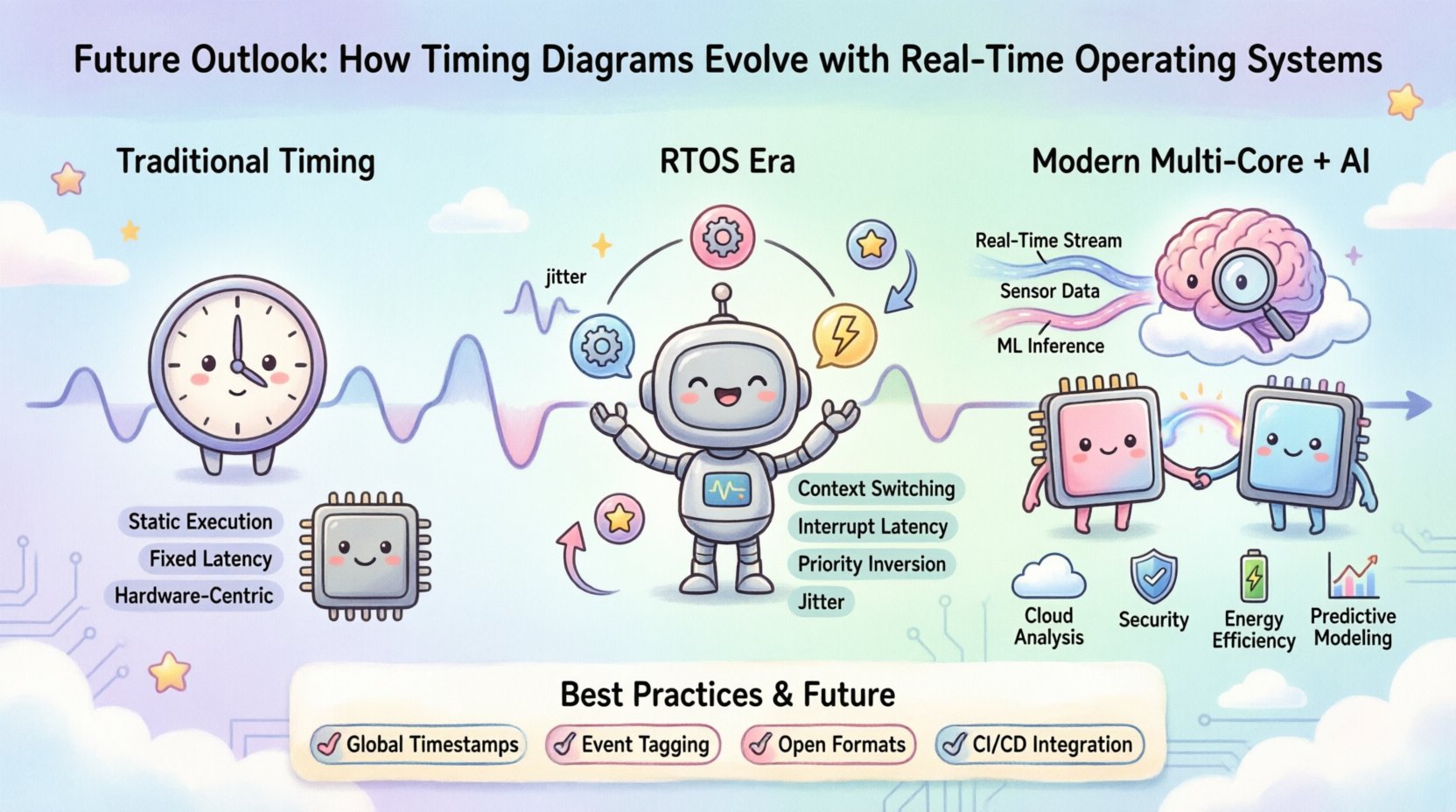
📜 The Traditional Timing Diagram Landscape

Historically, timing diagrams focused on hardware signal integrity. Engineers used them to verify clock cycles, setup times, and hold times. The relationship between the processor and peripherals was often treated as a fixed sequence. This approach worked well for bare-metal firmware where code executed in a predictable loop.

• Static Execution: Code ran sequentially without interruption.
• Fixed Latency: Delays were constant and calculable.
• Hardware-Centric: Focus was on electrical timing rather than task scheduling.

As software complexity grew, these diagrams became insufficient. They could not represent the non-deterministic nature of modern multitasking environments. The introduction of operating systems meant that multiple tasks competed for resources. This competition required a new way to visualize time.

⚙️ The RTOS Impact on Signal Correlation

Real-Time Operating Systems manage multiple threads or tasks concurrently. This introduces a layer of abstraction between the physical hardware and the logical application. Timing diagrams must now account for the scheduler’s decisions. When a high-priority task interrupts a low-priority one, the timeline shifts abruptly.

Key Challenges in RTOS Timing:

• Context Switching Overhead: Saving and restoring state takes cycles. This adds invisible time to the execution path.
• Interrupt Latency: The delay between an interrupt request and the service routine start.
• Priority Inversion: A high-priority task waits for a resource held by a lower-priority task.
• Jitter: Variations in response time due to background system activity.

Visualizing these events requires granular trace data. Engineers must see not just what happened, but when it happened relative to the scheduler ticks. This level of detail was not necessary in single-threaded systems.

🔍 Challenges in Modern Multi-Core Architectures

The shift to multi-core processors has further complicated timing analysis. In a single-core system, only one instruction stream runs at a time. In a multi-core environment, tasks run in parallel. This introduces new synchronization issues that timing diagrams must represent.

Core Interaction Points:

• Cache Coherency: Data must be synchronized across cores. This creates bus contention.
• Inter-Processor Interrupts (IPIs): Messages sent between cores to coordinate work.
• Shared Memory Access: Race conditions can occur if locks are not managed correctly.
• Power Management: Dynamic frequency scaling affects timing predictions.

A timing diagram for a multi-core system is no longer a single timeline. It becomes a matrix of timelines. Each core has its own execution trace. Engineers must correlate events across these timelines to understand system behavior. This requires advanced visualization tools that can handle massive datasets.

🤖 Integration with AI and Machine Learning

Artificial Intelligence is beginning to influence how timing data is processed. Traditional methods rely on manual inspection of traces. Machine learning algorithms can automate anomaly detection. They can predict timing violations before they occur in production.

Applications of AI in Timing Analysis:

• Predictive Modeling: Estimating latency based on historical data patterns.
• Anomaly Detection: Identifying irregularities in interrupt handling.
• Optimization Suggestions: Recommending scheduling changes to reduce jitter.
• Automated Debugging: Correlating crash logs with timing events.

This integration allows for proactive system tuning. Instead of reacting to failures, engineers can optimize for worst-case execution time (WCET) more accurately. The diagrams themselves may evolve into dynamic models that update as the system learns.

📊 Comparing Visualization Approaches

Different methods exist for representing timing data. Each has strengths and weaknesses depending on the system architecture. The table below outlines the primary approaches used in modern development.

Approach	Best For	Limitations
Static Waveforms	Simple hardware interfaces	Cannot show runtime variability
Task Gantt Charts	RTOS scheduling analysis	Hard to correlate with hardware signals
Hybrid Trace Views	Complex multi-core systems	High data volume requires optimization
Statistical Histograms	Latency distribution analysis	Loses specific event context

Selecting the right approach depends on the specific verification goals. A hardware driver might need waveforms, while an application scheduler needs Gantt charts. The future lies in combining these views into a single interface.

🛠️ Best Practices for Visualization

To effectively utilize timing diagrams in an RTOS environment, teams should adopt specific practices. These steps ensure that the data remains useful and interpretable.

• Standardize Timestamps: Use a global time base across all cores and peripherals.
• Minimize Overhead: Trace buffers can slow down the system. Use sampling or event-driven recording.
• Tag Critical Events: Mark entry and exit points of critical sections clearly.
• Abstraction Layers: Separate hardware timing from application logic for clarity.
• Version Control: Treat timing data like code. Store changes over time to track regressions.

Following these practices reduces the cognitive load on engineers. It allows them to focus on the root cause of timing issues rather than deciphering the data format.

🔮 Looking Ahead: Future Standards

As systems grow more complex, standardization becomes crucial. Currently, many proprietary formats exist for trace data. This creates silos in the development workflow. Future trends point towards open formats for timing data.

Emerging Trends:

• Open Trace Formats: Standardized file structures for interoperability.
• Cloud-Based Analysis: Offloading heavy processing to remote servers.
• Real-Time Collaboration: Multiple engineers viewing the same trace simultaneously.
• Integration with CI/CD: Automated timing checks in the build pipeline.

This shift will make timing analysis more accessible. It will no longer be a specialized task for a few experts. Instead, it will become part of the daily workflow for all developers.

⚡ Energy Efficiency and Timing

Power consumption is a major concern in modern embedded design. Timing diagrams can also reveal energy inefficiencies. By analyzing idle states and wake-up events, engineers can optimize power usage.

Power-Timing Correlations:

• Idle Periods: Longer idle times allow for deeper sleep modes.
• Wake-Up Latency: Faster wake-up reduces energy wasted in transition states.
• Bus Activity: Reducing unnecessary bus transactions saves power.

Timing diagrams help identify where energy is being wasted. This is vital for battery-operated devices. It bridges the gap between performance and longevity.

🛡️ Security Implications

Security is increasingly tied to timing behavior. Side-channel attacks rely on measuring execution time to infer secret data. Timing diagrams can help detect these vulnerabilities.

Security Considerations:

• Constant Time Execution: Ensuring operations take the same time regardless of input.
• Timing Side-Channel Detection: Identifying leaks in cryptographic routines.
• Denial of Service: Preventing tasks from monopolizing time slices.

By visualizing timing at a granular level, security flaws become visible. This integration of security and timing analysis is a growing necessity.

🏁 Final Thoughts on System Design

The evolution of timing diagrams reflects the broader trends in computing. We are moving from simple, linear processes to complex, distributed systems. The tools we use must evolve to match this complexity.

Real-Time Operating Systems introduce a layer of abstraction that demands more sophisticated analysis. Engineers must look beyond simple waveforms to understand the dynamic behavior of the kernel. Multi-core architectures add another dimension, requiring correlation across multiple timelines.

Adopting new visualization techniques and standards will improve the reliability of embedded systems. It will also enhance security and energy efficiency. As the industry moves forward, the timing diagram remains a vital artifact. It provides the clarity needed to navigate the complexity of modern hardware.

Staying informed about these developments is essential. The field is changing rapidly. Continuous learning ensures that designs remain robust. By focusing on accurate timing analysis, teams can build systems that are safe, efficient, and reliable.

The future of timing diagrams lies in integration. Combining hardware, software, and AI into a unified view offers the best path forward. This holistic approach will define the next generation of embedded design.